Monday, December 17, 2012

Image Compression using DCT (Discrete Cosine Transform)

It has been a while , so I decided to write something from memory to keep this blog alive. Currently I am stuck with some differential equations,i really want to solve that by hand. The more i dig, it becomes more complicated.

DCT aka Discrete Cosine Transform is similar to Fourier transform but uses only Cosine functions.
Its output is just scalar values , not complex numbers as in Discrete Fourier Transform. In image processing point of view it can be used to compress data. Jpeg format uses this technique to compress data. Besides this you can use this property to any field , where you want to get only some influencing data out of your sample.

There exists different kind of kernel functions for DCT. Out of which common form is shown below.
X_k =
 \sum_{n=0}^{N-1} x_n \cos \left[\frac{\pi}{N} \left(n+\frac{1}{2}\right) k \right] \quad \quad k = 0, \dots, N-1.

I copied this from wiki. If you carefully examine you can visualize this as projecting your data on the cosine.

Let us now apply DCT over an array of numbers
result = FourierDCT[{1, 10, 2, 3, 4, 2, 5, 7, 2, 10, 10, 11, 2}]
{19.1372, -3.7222, 1.37076, 2.10949, -2.33856, 2.01418, -4.42612, 0.769566, -2.33272, -3.44945, -3.3978, 1.07119, -2.33659}

This is the result , now lets take only first 10 from result array. That is .
len = Length[result];  // assign length (13) to variable len.
compressed  = Take[result, 10]

{19.1372, -3.7222, 1.37076, 2.10949, -2.33856, 2.01418, -4.42612, 0.769566, -2.33272, -3.44945}

Now lets take Inverse DCT of this compressed data which is expected to give our valuable original data back. Note original array 'result' contained  13 numbers  So we need to fill the remaining items with 0's.

FourierDCT[PadRight[compressed, len], 3];
This will output as below.
{1.682, 8.26, 4.01, 1.549, 4.43, 2.42, 4.41, 6.876, 3.40, 7.369, 13.12, 8.47, 2.96}
Note the similarity with original data , We just did a simple compression on input data and recovered successfully. This is a lossy compression technique. Applying this on image will not reduce the overall quality of image. I mean it is still possible to understand the original image.

Let us now apply this example on an image. This is our original image, Did you able to recognize him? if you are a German you must. He is the prince of mathematicians.

This image's dimensions is {220,282} and GrayScale.

Lets now take only first 100 rows from this image and compress it


dctResult = FourierDCT[ImageData[ image, "Byte"]];
Length[dctResult];
// Here we are only taking first 100 rows from image , that is we are compressing it
compressed = Take[dctResult, {1, 100}];

Now let us recreate this compressed data again , and see how it looks like
padded = PadRight[compressed, {282, 220}];
resImage = FourierDCT[padded, 3];
Image[resImage, "byte"]


It is not that bad, still you can recognize him.
How about taking 200 rows from the original image. See the output below . It is actually good. We just saved (282-200) * 220 bytes by this simple compression. (282 is original image height, 220 is width)


I used mathematica program here. Hopes still you could get the idea.
Now again , I am asking , Did you recognize this genius ? if not he is Carl Friedrich Gauss, the Legend.

Wednesday, October 24, 2012

3D Face creation in Android

Before 3 weeks  one  thought came to my mind, like for creating a 3D surface/object for face image using Opengl ES- Android. Recently I got some time to implement that.

The the basic idea is like this. Create a mesh surface and texture map it with the image of the face which you want on  it. Then provide/implement some tools to bevel up/down on these mesh preserving the smoothness of the surface. I don't want to mention too much details here, because i don't think it contains enough theories which needs explanation.

See the video below( taken with a web cam). May not have enough clarity. I implemented this app in Java only and it took almost 6 hours. After creating the 3D face object ,App will allow user to export it as OBJ format. But that part needs to be done and i am lazy. So Ii stopped further implementation :)


Is anybody  interested in the code?   ;). 

Wednesday, August 15, 2012

Bending Energy Continued - Finding K


In the previous post I showed how to find F'(s) of a a curve F(t) = <X(t),Y(t),Z(t)>

Now according to the definition of bending energy , it is the integrated sum of squares of curvature over length of the curve. That is we need to find the curvature K(s). It is always like this , Just getting better and better! .

Curvature is the rate of change magnitude of Unit tangent vector with respect to curve length
That is , it is

K(s)  = || dF'(t) / ds ||

Lets find dF'(t) / ds

This is (dF'(t)/ dt) * (dt/ ds)   using chain rule of diff.

=   || dF'(t) / dt ||
    -----------
      || ds/ dt      ||       we know ds/dt = || F'(t) ||  from previous post. and dF'(t)/dt is F''(t) .

K(t)  = || F''(t) || /  || F'(t) ||

we calculated the value of K(t).  For curves like circle , K(t) is same everywhere ,so just we can remove parameter t for circle. Also for circle there is exists an easier fomula : K = 1 / radius.

Sunday, August 12, 2012

Bending Energy & Parameterization of Curve over length


What is bending Energy  ? The precise definition is "it is the sum of squares of curvature of the curve function parameterized over curve length". Bending energy gives the energy stored in the curve. We know any bented objects will store some energy. Bending energy formulation helps to find a value proportional to the energy stored in the curve. For a straight line  bending energy is Zero.

 Before look into it we need to understand how we can parametrize curve over length

The tricky part is how we can parameterize over curve length.

Consider a vector valued function F(t) =  < X(t),Y(t),Z(t) > , t is the parameter , ranges between some values.

F'(t) can be found easily by applying partial differentiation on F with respect to 't' .

Lets now find the length (length function) of this curve


it has been shown by Kennedy, John (2011) in his paperhow to derive expression for F'(s)

Differentiating this with respect to s , we will get

1 = || F'(s) ||  (of-course s is based on t)

That means after changing the parameter from t to s(length param) the length of F'(s) is getting 1. It is very interesting concept, that means on moving through function F(S) we are moving exactly by unit length. If you  imagine this it seems true. Because no matter where the curve is going its length get incremented in equal length.

So how we can find the equation for F'(s) ? Intuitively we can think like this. Anyway F(s) and F(t) represents  same curve  , only different is magnitude of F'(s) is 1 , But F'(t) may not be 1. But both these vectors points to the same direction. right ? so we(I)can conclude like this

   F'(s) = F'(t) / || F'(t) ||


Other-way is like this.


Now Differentiating both sides with respect to t.

ds/dt = || F'(t) ||

If we differentiate  function F(t) with respect to s (length) we get

= F'(t) * dt/ds (chain rule of differentiation)
= F'(t) / (ds/dt)
= F'(t) / || F'(t) || ( we know ds/dt = || F'(t) || )

that is  dF(t)/ds =  F'(t) / || F'(t) which is eqult to F'(s). This is fantastic. :)

Now Next step is finding F''(s) , I will explain that in next post. It is time to sleep.
Nowadays days I am getting more into mathematics than software engineering. To really understand things you need to have great patience and curiosity.  After all these years , I am still a novice.


Monday, July 16, 2012

First steps into Robotics.


First steps into Robotics.

Yes , I decided to start looking into the interesting Robotics domain. Since i am not an electronics/mechanical engineer, i don't have any plan to build my own 'kd' Robot. My interest is in computer vision. I just want to study how these systems can be practically implemented. Like how we can program a small car for automatic parking on your Dining table!.

For starters , it is difficult to find some good starting point.
IF you have money to spend , you can buy eddie , Which supports microsoft RDS.
Following picture shows eddie.


For others, there are couples of basic robots like Boe-Bot which is cheaper and has some basic sensors.


mmm... Thats all for now. God knows how will it ends up.

Wednesday, April 18, 2012

Frequency Identification

In this post i will try to explain the basic things to identify major frequency components from a data.This helpful filtering certain frequencies from the source or for doing some analysis. Frequency analysis a must learn thing if you are learning image processing, signal processing.
 Basic idea is to convert the data to frequency domain using discrete fourier transformation, and using that we can find the major frequency in the data.Before going to the details lets look the equation of a basic Sin wave

it is sin( 2*Pi/T * t )
where T is the time period of wave
            t is the instantaneous  time.
            Pi Ofcourse 22/7 , 
Lets plot this wave. I am using mathematica to plot the wave. 
Here is the wave form
T = 20
Plot[ Sin[2*Pi/T*t], {t, 0, 50}] . (We can verify T =20 from the graph.)


So the frequency of this wave is 1/T . that is 1/20.
Ok.  this is no big deal unless you are very weak in mathematics. Now lets add some random noise to it

n = 1500;
T = 20;
SampledData= Table[Sin[2 Pi* x/T] + RandomReal[.8], {x, n}] ;
ListLinePlot[SampledData]


I hope now you cannot identify the frequency from this ;) .Lets find the T period from this , it must approximate to 20.Before that lest look the equation of one dimensional DFT

Where N is the total number of elements and k/N will give the frequency (because Sin (2*Pi*f * n ) .Ok , now i am going to do DFT with data generated with equation Sin[2 Pi* x/T] and I am  going to find the power spectrum(magnitude of complex numbers)

DftData = Abs[Fourier[SampledData]];

lets plot the power spectrum graph


In graph you can see two spikes. The rightmost spike represent the nyquest frequency( i will explain it later). lets find the first position where magnitude is highest.

pos = Position[f, Max[f]][[1, 1]]
it will be at 76.

Now we can find the frequency by substituting this value for k in equation k/N .
that is 76/1500 = .0506. which approximates to 1/20.

If you want to find the timer period just find the reciprocal. 
T = 1500/76 = 19.73!! approximates to 20.

Hey you just learnt a great thing!!. 

Thursday, April 12, 2012

MD2 animation

Before 2 weeks I added Md2 animation support to my engine. It was an easy task. MD2 has some predefined set of animations. MD2 is used by games like QuakeII,Sin, Solider Of Fortune .

See the  MD2  animations running with my engine(Video lacks clarity because my screen capture software not allows to record at high frame rate with good quality)


While coding MD2 loader i found that the skin path in the MD2 file is relative and sometimes entirely in some other directory. So we cannot rely on this path. In MD2 file they are trying to minimize the model data by using different techniques like having predefined normal vector set. The creators also store texture coordinates as short rather than float.you need to divide by the size of texture to get the real texture uv coordinates.

One other problem is with inconsistent naming convention of frames. say we have 120 frames , and in one Md2 file 10-20 frames contains animation for running data with name "Run001", but in some other file they use "Run__1"..  it would be better if the creators have made a standard for frame names.

Finally you can use blender modeler software to create MD2 animations.(i heard it is buggy :) , Thats ok Bugs are everywhere), 

Wednesday, April 11, 2012

Gaussian filter


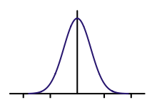
Gaussian Filter modifies the input data by convolution with a Gaussian distribution. Gaussian filter is often used to smooth out images.In this post i will try to show the frequency response of Gaussian filter.  It is very important to understand the frequency domain behaviorism.When we consider the frequency response of gaussian one diamension filter we can see that , the filter reponse is inversely proportional to the frequency, lower the frequency, its response is high, that is more smoothing happens to lower frequency components.

An unnormalized Gaussian distribution is 

where is the standard deviation. This function is will form a belll shaped curve with center at 0.  This function is non zero every where(high value at center and decreases ). curve is shown below
A normalized gaussian distribution can be found by normalizing the above equation with the total area, which can be found by integrating it over -Infinite to +infinite. 


so the normalized equation is(from wiki) : g(x) = \frac{1}{\sqrt{2\cdot\pi}\cdot\sigma}\cdot e^{-\frac{x^2}{2\sigma^2}}


Frequency response of a 1-D Gaussian filter can be found by doing DFT over the 1-D kernel,

We can find it in mathematica simply with following commands

 DftResults =    Fourier[   Table[PDF[NormalDistribution[0,1],x],{x,-3,3,.01}] ];
 ListLinePlot [ Abs[DftResults],PlotRange->All ]

This will plot the power spectrum of Gaussian 1-D filter. It will look like this (X axis-frequency,Y axis magnitude), we can see that at lower frequency level , filer gives better output.. the extreme right shows the nyquist frequency( ignore that for now. ). From this we can see Gaussian filter act as a low pass filter.


Monday, January 23, 2012

GFD(Generalized Fourier Descriptor), Part 1

it is interesting.. GFD is a rotation invariant. In GFD the orginal image is transformed to polar cordinate system. This provides the rotation invariant ability. I will explain how this happens. When we map normal image in cartesian coodinate system to polar coordinates, a rotation in Cartesian coordinate will cause translation/shifting in polar system. Remeber in polar system r, and theta are the axis. So when you rotate original image, R remain same so in effect the coresponding image is shifted(to left/right according to the direction of rotation) in polar system.

Still you may be wondering even if that is the case, why Fourier transform output remains same ? because we are operating on different data.For each rotation , the image is shifted in polar coordinate system.
If you thought like that, you are thinking.. Good.

I will explain the answer to the above puzzle.

X_k = \sum_{n=0}^{N-1} x_n \cdot e^{-i 2 \pi \frac{k}{N} n}.

If you remember one dimensional Fourier transform you can see that we are finding the dot product of our Image data with a number of Cos,Sin vectors (N diamensional, same as image size). The sin and cos are orthonormal , so the magnitude remains same. Please read my previous post http://cgmath.blogspot.com/2011/12/image-recognition-using-phase-only.html to get an intuitive grasp on DFT.

that is

Magnitude Of DFT[ {1,2,3,4,5,6}] is equal to Magnitude of DFT[ {4,5,6,1,2,3}]

Magnitude is Sqrt( i*i + j*j ) of the complex number.

Thus we get rotation in-variance. Now the next thing is Fourier descriptor. I will post about that after some days. It is simple( Really ? )


Tuesday, January 10, 2012

Just started with generalized Fourier Descriptor

I started working on a new algorithm for image search. This is based on Fourier descriptor. Image is first converted in to a corresponding polar representation.This representation allows to get complete rotation in-variance. This is Because a rotation in Cartesian plane corresponds to a angle shifts in polar domain. So the DFT remains same. This is a simple and great idea.

I also started working on my Engine to add MD2 animation support. The image processing things takes too much thinking time also sometimes makes me dull. Thats why i started this to feed my interests.MD2 animation is simple to implement also to understand. Bone animation is difficult to understand if you are a beginner/intermediate in computer graphics. You may be wondering about which format should be used like that.. I had a looked that before some years. But at that time i didn't got time to implement it. Now sadly i am not remembering much.I should have implemented it that time.