Thoughts about Regression analysis

Recently i watched a video about regression and probability, Here i am presenting some information from that.

Regression analysis is about establishing relationship between variables. That means there will be set of independent variables and corresponding dependent variables.

Example

let us denote price of a house using variable Y and factors affecting the price, such as area,age,location using variable X.

To make everything more simpler, let us take only the area of house as the independent variable, so there will be only one feature. Now we need to model the price (Y) of house. So that we can predict the price of an house if someone gives us the area. We can use the following simple equation to model that

H(t0,t1,i) =  t0 + t1 * X(i)  ----------------->  EQ(1)

t0 and t1 are constants.. ( when we have multiple factors, deciding the price other than area then it is possible to add more features to equation like  't0 + t1 * X1 + t2 * x2 + t2 * X1 * X2' or so on)

X(i) indicate sample number. That means if we have 100 data set containing 'area - price' pairs then X(5) will indicate the 5th area from the given data set.

If we plot EQ1(1), it will be a line for sure. So basically we are trying to find a line which will match with the expected set of house prices. See the following image.. where you can see a line which can be used to predict house price on a X value.





EQ(1) can be changed to higher degrees to achieve more complex predictions.  But simply adding more degrees will not help much. You also need to define the model in a more meaningful way.

Back to problem,
Now we need to find values for 't0' and 't1'  such that it will help to form a meaningful model.
For that we need to define cost function



-------------  EQ(2)



From EQ(2) we can see that , it is actually finding the sum of squared difference between expected value and our defined model (here it is based on line equation).

Aim must be to minimize EQ(2) , more we can minimize, less error will be , and our predicted line will be aligned more closely to the price data set. To do that we can use gradient descent method (other complicated solutions are also avilable, like conjugate gradient descent or BFGS , these are better than simple gradient descent , but complex to implement).

So for implementing gradient descent we need to find the gradient of function J with respect to t0 and t1 . You can use matlab to find that or find it manually. Following are the results



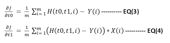
Now apply gradient descent to minimize function J.  Below shown the steps to do this in matlab.

% X valuessampleX = [ 0 1 2 3 4 5 6 7 8 9 10 11 12 13 14 15 16];% Y valuessampleY = [100 110 120 122 125 135 112 122 128 129 130 124 117 116 128 132 125];
% Y predicted using final model.resultY = [sampleY ];ss = size(sampleY);m = ss(2);resultC = zeros(ss(2),3);
cmap = hsv(1);
error = [];
theta0 = 50;theta1 = 1;
% main iteration loopfor i = 1:1:10000
% function HnewSampleY = theta0 + theta1 * sampleX;
deviation = sum((newSampleY - sampleY).^2);deviation  = deviation / (2*ss(2));error = [ error ;deviation ];
resultY = [newSampleY];colorPoints = zeros(m,3);colorPoints(1: end,1) = cmap(1,1);colorPoints(1: end,2) = cmap(1,2);colorPoints(1: end,3) = cmap(1,3);%resultC = [resultC;  colorPoints];resultC = [ colorPoints];
% derivative of J w.r.t t0theta0Gradient = sum(newSampleY - sampleY) / m;% derivative of J w.r.t t1theta1Gradient =  sum((newSampleY - sampleY).*sampleX ) / m;
% applying gradient descent operation to minimize Jtheta0 = theta0 - .01 * theta0Gradient;theta1 = theta1 - .01 * theta1Gradient;
end 

scatter([sampleX sampleX],[sampleY resultY],[],[ zeros(m,3);  resultC]);axis([0 50 -100 100]);hold; 
fprintf('\ncomputed error values\n');error

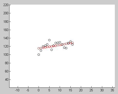
Below image show the result after running this code. Red circles indicate the points generated using final model, black circles indicates the input data.



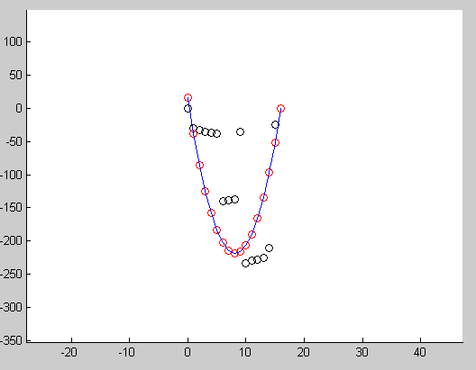
Another example showing how we can use this to fit a quadratic curve to input points.

Implicit surfaces and Level Set

Things are more complicated in discretized form. Say a line when discretized is not actually a line, Right(remembering the bresenham line algorithm ) ? Same thing goes to circle or any shapes. So for computing the associated properties we need more techniques. Implicit surface helps us to compute such properties.

Before I explain about implicit surfaces, you tell be what is the gradient of a scalar surface/curve.
Say you define a 3D surface by the equation x*x + y*y + z*z = 9, we can easily see that this surface is nothing but a sphere with radius 3. Right ?
So Q(x,y,z) = x*x + y*y + z*z - 9 = 0.
What is the gradient of Q then ? it represents the normal at any point on this surface , and it is (2x,2y,2z) (not normalized).

Why i said this was to show you how easy it is compute the gradient of a surface with an explicit equation. We can also easily compute other properties related with that surface like tangent,curvature,etc.

But what can you do if you don't have such explicit equations. In practical things will be like this.
In Implicit form we can define a shape implicitly. Our shape must be closed and non-self intersecting. With this agreement we can define the shape with following definitions.

Let P ( { Xi,Yi } ) be our point set which denotes the boundaries of our shape. We can define shape implicitly based on the following conditions.

1. For all points in shape boundaries ∅ (Pi) = 0
2. For all other points outside the shape ∅(Pi) must be > 0 
3. For all other points inside the shape ∅(Pi) must be < 0 . (Conditions 2,3 can be interchanged though) 

Based on the earlier definitions consider the above picture. Pixel's with green boundary is our shape where ∅(Pi) will be 0. pixels having red color will have negative value, and rest of the pixels (blue) will have positive value. This is how we define implicit functions for complicated shapes. In the next post I will show you how we can numerically compute the properties of these shapes from this definitions also will introduce about level sets. It is not a big deal( Actually i had intention to write more about this, but I lost my mood so stopping now )

Curvature Flow & Smoothing curves

I am getting addicted to curves. They are the perfect beautiful representation which we can numerically compute. I don't want to express more my feelings towards it which may be boring to you.

Coming to the topic, curvature flow is a kind of method to modify the curve.
Take any planar non intersecting curves , find the curvature at each point and multiply with it the normal there, then move the curve along that direction. This is the concept. It is analogs to the heat exchange. Heat will eventually spread uni-formally , no matter how you wrap it.

So take a curve {X(s),Y(s)} and it's curvature and normal , Say  {K(s)} and {N(s)}.
Then curvature flow vector is defined as {K(s)*N(s) }.

Using this technique we can smooth the curve from noise. Eventually this curve will become circular and will vanish. it is possible to know the exact point where it will vanish.

I just made a quick demo of this with matlab. See the images below

Original curve.
We can see that some edges are not smooth (think of it like created by noise).These spikes(non-smooth) in edges are not influencing our capability to detect the shape.We humans normally pick up a smooth shape from a contour. Now we want to remove some noise (or say smooth it) using curvature flow.

After 10 iteration

See that curve is more smooth now.

Curve after 50 Iterations
Curve is getting circular. Yeah, it will become circular at one point , because circle is the only one shape with a non-zero uniform curvature.

This is type of smoothing is also possible with Gaussian filtering along the curve,but with lesser accuracy. This type of technique can also be extended to 3D, Say you are having an object and you want to add a higher layer of layer/cover to it. Rather than just extending the surface along normal , use curvature flow.Then the surface will be more appealing and natural (I Guess).