Wednesday, April 18, 2012

Frequency Identification

In this post i will try to explain the basic things to identify major frequency components from a data.This helpful filtering certain frequencies from the source or for doing some analysis. Frequency analysis a must learn thing if you are learning image processing, signal processing.
 Basic idea is to convert the data to frequency domain using discrete fourier transformation, and using that we can find the major frequency in the data.Before going to the details lets look the equation of a basic Sin wave

it is sin( 2*Pi/T * t )
where T is the time period of wave
            t is the instantaneous  time.
            Pi Ofcourse 22/7 , 
Lets plot this wave. I am using mathematica to plot the wave. 
Here is the wave form
T = 20
Plot[ Sin[2*Pi/T*t], {t, 0, 50}] . (We can verify T =20 from the graph.)


So the frequency of this wave is 1/T . that is 1/20.
Ok.  this is no big deal unless you are very weak in mathematics. Now lets add some random noise to it

n = 1500;
T = 20;
SampledData= Table[Sin[2 Pi* x/T] + RandomReal[.8], {x, n}] ;
ListLinePlot[SampledData]


I hope now you cannot identify the frequency from this ;) .Lets find the T period from this , it must approximate to 20.Before that lest look the equation of one dimensional DFT

Where N is the total number of elements and k/N will give the frequency (because Sin (2*Pi*f * n ) .Ok , now i am going to do DFT with data generated with equation Sin[2 Pi* x/T] and I am  going to find the power spectrum(magnitude of complex numbers)

DftData = Abs[Fourier[SampledData]];

lets plot the power spectrum graph


In graph you can see two spikes. The rightmost spike represent the nyquest frequency( i will explain it later). lets find the first position where magnitude is highest.

pos = Position[f, Max[f]][[1, 1]]
it will be at 76.

Now we can find the frequency by substituting this value for k in equation k/N .
that is 76/1500 = .0506. which approximates to 1/20.

If you want to find the timer period just find the reciprocal. 
T = 1500/76 = 19.73!! approximates to 20.

Hey you just learnt a great thing!!. 

Thursday, April 12, 2012

MD2 animation

Before 2 weeks I added Md2 animation support to my engine. It was an easy task. MD2 has some predefined set of animations. MD2 is used by games like QuakeII,Sin, Solider Of Fortune .

See the  MD2  animations running with my engine(Video lacks clarity because my screen capture software not allows to record at high frame rate with good quality)


While coding MD2 loader i found that the skin path in the MD2 file is relative and sometimes entirely in some other directory. So we cannot rely on this path. In MD2 file they are trying to minimize the model data by using different techniques like having predefined normal vector set. The creators also store texture coordinates as short rather than float.you need to divide by the size of texture to get the real texture uv coordinates.

One other problem is with inconsistent naming convention of frames. say we have 120 frames , and in one Md2 file 10-20 frames contains animation for running data with name "Run001", but in some other file they use "Run__1"..  it would be better if the creators have made a standard for frame names.

Finally you can use blender modeler software to create MD2 animations.(i heard it is buggy :) , Thats ok Bugs are everywhere), 

Wednesday, April 11, 2012

Gaussian filter


Gaussian Filter modifies the input data by convolution with a Gaussian distribution. Gaussian filter is often used to smooth out images.In this post i will try to show the frequency response of Gaussian filter.  It is very important to understand the frequency domain behaviorism.When we consider the frequency response of gaussian one diamension filter we can see that , the filter reponse is inversely proportional to the frequency, lower the frequency, its response is high, that is more smoothing happens to lower frequency components.

An unnormalized Gaussian distribution is 

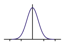
where is the standard deviation. This function is will form a belll shaped curve with center at 0.  This function is non zero every where(high value at center and decreases ). curve is shown below
A normalized gaussian distribution can be found by normalizing the above equation with the total area, which can be found by integrating it over -Infinite to +infinite. 


so the normalized equation is(from wiki) : g(x) = \frac{1}{\sqrt{2\cdot\pi}\cdot\sigma}\cdot e^{-\frac{x^2}{2\sigma^2}}


Frequency response of a 1-D Gaussian filter can be found by doing DFT over the 1-D kernel,

We can find it in mathematica simply with following commands

 DftResults =    Fourier[   Table[PDF[NormalDistribution[0,1],x],{x,-3,3,.01}] ];
 ListLinePlot [ Abs[DftResults],PlotRange->All ]

This will plot the power spectrum of Gaussian 1-D filter. It will look like this (X axis-frequency,Y axis magnitude), we can see that at lower frequency level , filer gives better output.. the extreme right shows the nyquist frequency( ignore that for now. ). From this we can see Gaussian filter act as a low pass filter.