Thoughts about Regression analysis

Recently i watched a video about regression and probability, Here i am presenting some information from that.

Regression analysis is about establishing relationship between variables. That means there will be set of independent variables and corresponding dependent variables.

Example

let us denote price of a house using variable Y and factors affecting the price, such as area,age,location using variable X.

To make everything more simpler, let us take only the area of house as the independent variable, so there will be only one feature. Now we need to model the price (Y) of house. So that we can predict the price of an house if someone gives us the area. We can use the following simple equation to model that

H(t0,t1,i) =  t0 + t1 * X(i)  ----------------->  EQ(1)

t0 and t1 are constants.. ( when we have multiple factors, deciding the price other than area then it is possible to add more features to equation like  't0 + t1 * X1 + t2 * x2 + t2 * X1 * X2' or so on)

X(i) indicate sample number. That means if we have 100 data set containing 'area - price' pairs then X(5) will indicate the 5th area from the given data set.

If we plot EQ1(1), it will be a line for sure. So basically we are trying to find a line which will match with the expected set of house prices. See the following image.. where you can see a line which can be used to predict house price on a X value.





EQ(1) can be changed to higher degrees to achieve more complex predictions.  But simply adding more degrees will not help much. You also need to define the model in a more meaningful way.

Back to problem,
Now we need to find values for 't0' and 't1'  such that it will help to form a meaningful model.
For that we need to define cost function



-------------  EQ(2)



From EQ(2) we can see that , it is actually finding the sum of squared difference between expected value and our defined model (here it is based on line equation).

Aim must be to minimize EQ(2) , more we can minimize, less error will be , and our predicted line will be aligned more closely to the price data set. To do that we can use gradient descent method (other complicated solutions are also avilable, like conjugate gradient descent or BFGS , these are better than simple gradient descent , but complex to implement).

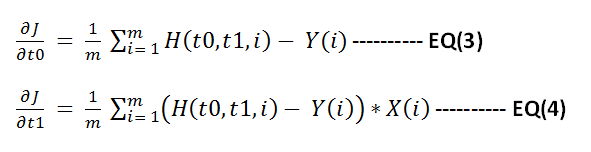
So for implementing gradient descent we need to find the gradient of function J with respect to t0 and t1 . You can use matlab to find that or find it manually. Following are the results



Now apply gradient descent to minimize function J.  Below shown the steps to do this in matlab.

% X valuessampleX = [ 0 1 2 3 4 5 6 7 8 9 10 11 12 13 14 15 16];% Y valuessampleY = [100 110 120 122 125 135 112 122 128 129 130 124 117 116 128 132 125];
% Y predicted using final model.resultY = [sampleY ];ss = size(sampleY);m = ss(2);resultC = zeros(ss(2),3);
cmap = hsv(1);
error = [];
theta0 = 50;theta1 = 1;
% main iteration loopfor i = 1:1:10000
% function HnewSampleY = theta0 + theta1 * sampleX;
deviation = sum((newSampleY - sampleY).^2);deviation  = deviation / (2*ss(2));error = [ error ;deviation ];
resultY = [newSampleY];colorPoints = zeros(m,3);colorPoints(1: end,1) = cmap(1,1);colorPoints(1: end,2) = cmap(1,2);colorPoints(1: end,3) = cmap(1,3);%resultC = [resultC;  colorPoints];resultC = [ colorPoints];
% derivative of J w.r.t t0theta0Gradient = sum(newSampleY - sampleY) / m;% derivative of J w.r.t t1theta1Gradient =  sum((newSampleY - sampleY).*sampleX ) / m;
% applying gradient descent operation to minimize Jtheta0 = theta0 - .01 * theta0Gradient;theta1 = theta1 - .01 * theta1Gradient;
end 

scatter([sampleX sampleX],[sampleY resultY],[],[ zeros(m,3);  resultC]);axis([0 50 -100 100]);hold; 
fprintf('\ncomputed error values\n');error

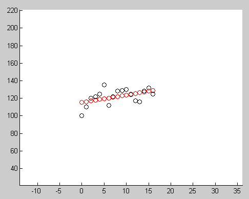
Below image show the result after running this code. Red circles indicate the points generated using final model, black circles indicates the input data.



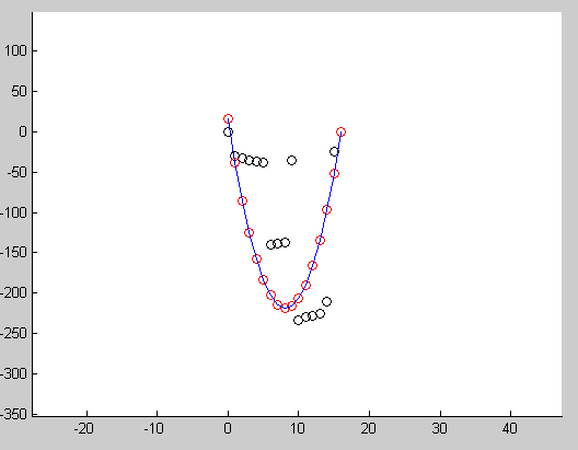
Another example showing how we can use this to fit a quadratic curve to input points.

Wiener Deconvolution: Deriving the final formula

Recently i watched a video which talks about noise and filtering.That why i am posting this.After searching the same in wiki, i didn't see a detailed derivation of the formula. so I thought to write this and post.

Wiener deconvolution is a frequency domain technique which helps to remove the noise if we know the degradation function(H(t)) in advance. The degradation function degrades the image quality. It can be blurring like Gaussian blur or it can be motion blur.

X(x,y) -> Passes through degradation function ->  Some noise gets added here(N) -> our final signal Y(x,y)

If we multiply the Y with Wiener filter then it will provide an approximation of X. Lets call this approximation as X$ .Now am going to write down the full derivation. a part of this is available in wiki. But those who are not remembering complex number maths may find it difficult.

Mean square error between approximation and original data is = E | X(x,y) - X$(x,y) | ^2

but we know X$ is  can be obtained by G(x,y) * Y(x,y)  [ * is convolution operator ]
 = E( | X(x,y) -  G(x,y) * Y(x,y)  |^2)
But if convert all to frequency domain convolution becomes multiplication, ie a(t)*b(t) = a(f)b(f)
Also we know Y is X * H + N
= E(| X -  G ( XH + N)) |^2)
= E(| X -  GXH - GN) |^2)
= E(| (1 -  G H)X - GN) |^2)

if A and B are two complex numbers | A B |^2 = (A B)(AB)* , here * is complex conjugate.

= E(  ((1-GH)X - GN)((1-GH)X - GN)* )
= E(  ((1-GH)X - GN)((1-G*H*)X* - G*N*)) , here all * means complex conjugate

Expanding this is a painful thing. but i am not giving up. So are you ?

= E( ((1-GH)X(1-GH)* XX* - (1-GH)XG*N* - GN(1-GH)*X* + GNG*N* )
= ( (1-GH)(1-GH)* E{|X|^2} - (1-GH)G* E{XN*} - G(1-GH)* E{NX*} + GG* E{|N|^2}
wooha,
Lets assume noise and input signal has no relation,That why it is noise. So we can just ignore the terms E{XN*} ,E{NX*}.I think this is because at a particular frequency we can't find any relation between input data and noise. So the probability is null here. That why taking E( expectation) which sums the probability of values. here since we can't find any probability we can assume it 0.

We can denote S(f) = E{|X|^2} , it is the power spectrum of the complex values of the input data
We can denote N(f) = E{|N|^2} , it is the power spectrum of the complex values of the noise  data

so final equation becomes

minError(f) =  (1-GH)(1-GH)* S + GG*N
Now we need to find the minimum error which we can obtain for G. So following the basic calculus (like how we will find the min value of a function ) . careful about G* ,it is not G. So we can treat that as constant.

d(minError(f)/dG = -H(1-GH)*S + G*N = 0 ,
Now we need to find G from this. we will find it in a minute.


That is  G*N - H[1-GH]*S = 0

G*N = HS[1-GH]*
G*N = HS[1-G*H*]
G*N = S[H-G*HH*]
G*N = S[H-G*|H|^2 ]
G*N = SH-SG*|H|^2 ]
G*N = (G*) [ (1/G*)SH-S|H|^2 ]
N = [ (1/G*)SH - S|H|^2 ]
N + S|H|^2 = SH/G*
G*/SH  = 1/ (N+ S|H|^2 )
G* = SH / ( N+  S HH* ).         Take out s
G* =  SH / S( N/S+ HH* )

N/S is noise to signal ratio, We can replace it with a constant K

G* =  H / (K+ HH* )
G   = H*/ (K+H*H), H*H is |H|^2|
G   = H*/ (K+|H|^2)

Yes we reached the final answer , G = H*/(K+|H|^2).
if you know H, then you can find G, Then just multiply this with Fourier transformed input data. you will get a better picture. Thus you can remove some noise from the input data. In next post i will try to post some samples after applying G or wiener filter. Be ready for it.