Thoughts about Regression analysis

Recently i watched a video about regression and probability, Here i am presenting some information from that.

Regression analysis is about establishing relationship between variables. That means there will be set of independent variables and corresponding dependent variables.

Example

let us denote price of a house using variable Y and factors affecting the price, such as area,age,location using variable X.

To make everything more simpler, let us take only the area of house as the independent variable, so there will be only one feature. Now we need to model the price (Y) of house. So that we can predict the price of an house if someone gives us the area. We can use the following simple equation to model that

H(t0,t1,i) =  t0 + t1 * X(i)  ----------------->  EQ(1)

t0 and t1 are constants.. ( when we have multiple factors, deciding the price other than area then it is possible to add more features to equation like  't0 + t1 * X1 + t2 * x2 + t2 * X1 * X2' or so on)

X(i) indicate sample number. That means if we have 100 data set containing 'area - price' pairs then X(5) will indicate the 5th area from the given data set.

If we plot EQ1(1), it will be a line for sure. So basically we are trying to find a line which will match with the expected set of house prices. See the following image.. where you can see a line which can be used to predict house price on a X value.





EQ(1) can be changed to higher degrees to achieve more complex predictions.  But simply adding more degrees will not help much. You also need to define the model in a more meaningful way.

Back to problem,
Now we need to find values for 't0' and 't1'  such that it will help to form a meaningful model.
For that we need to define cost function



-------------  EQ(2)



From EQ(2) we can see that , it is actually finding the sum of squared difference between expected value and our defined model (here it is based on line equation).

Aim must be to minimize EQ(2) , more we can minimize, less error will be , and our predicted line will be aligned more closely to the price data set. To do that we can use gradient descent method (other complicated solutions are also avilable, like conjugate gradient descent or BFGS , these are better than simple gradient descent , but complex to implement).

So for implementing gradient descent we need to find the gradient of function J with respect to t0 and t1 . You can use matlab to find that or find it manually. Following are the results



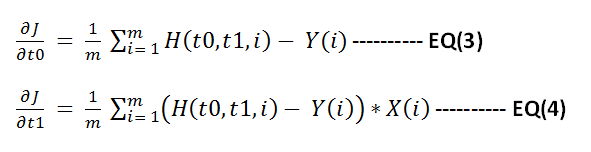
Now apply gradient descent to minimize function J.  Below shown the steps to do this in matlab.

% X valuessampleX = [ 0 1 2 3 4 5 6 7 8 9 10 11 12 13 14 15 16];% Y valuessampleY = [100 110 120 122 125 135 112 122 128 129 130 124 117 116 128 132 125];
% Y predicted using final model.resultY = [sampleY ];ss = size(sampleY);m = ss(2);resultC = zeros(ss(2),3);
cmap = hsv(1);
error = [];
theta0 = 50;theta1 = 1;
% main iteration loopfor i = 1:1:10000
% function HnewSampleY = theta0 + theta1 * sampleX;
deviation = sum((newSampleY - sampleY).^2);deviation  = deviation / (2*ss(2));error = [ error ;deviation ];
resultY = [newSampleY];colorPoints = zeros(m,3);colorPoints(1: end,1) = cmap(1,1);colorPoints(1: end,2) = cmap(1,2);colorPoints(1: end,3) = cmap(1,3);%resultC = [resultC;  colorPoints];resultC = [ colorPoints];
% derivative of J w.r.t t0theta0Gradient = sum(newSampleY - sampleY) / m;% derivative of J w.r.t t1theta1Gradient =  sum((newSampleY - sampleY).*sampleX ) / m;
% applying gradient descent operation to minimize Jtheta0 = theta0 - .01 * theta0Gradient;theta1 = theta1 - .01 * theta1Gradient;
end 

scatter([sampleX sampleX],[sampleY resultY],[],[ zeros(m,3);  resultC]);axis([0 50 -100 100]);hold; 
fprintf('\ncomputed error values\n');error

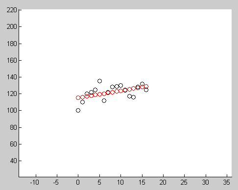
Below image show the result after running this code. Red circles indicate the points generated using final model, black circles indicates the input data.



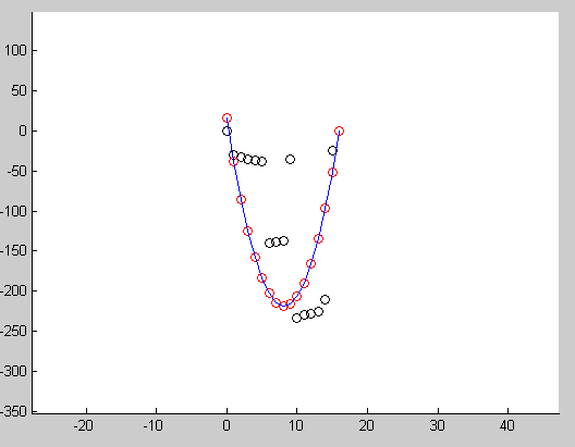
Another example showing how we can use this to fit a quadratic curve to input points.

Implicit surfaces and Level Set

Things are more complicated in discretized form. Say a line when discretized is not actually a line, Right(remembering the bresenham line algorithm ) ? Same thing goes to circle or any shapes. So for computing the associated properties we need more techniques. Implicit surface helps us to compute such properties.

Before I explain about implicit surfaces, you tell be what is the gradient of a scalar surface/curve.
Say you define a 3D surface by the equation x*x + y*y + z*z = 9, we can easily see that this surface is nothing but a sphere with radius 3. Right ?
So Q(x,y,z) = x*x + y*y + z*z - 9 = 0.
What is the gradient of Q then ? it represents the normal at any point on this surface , and it is (2x,2y,2z) (not normalized).

Why i said this was to show you how easy it is compute the gradient of a surface with an explicit equation. We can also easily compute other properties related with that surface like tangent,curvature,etc.

But what can you do if you don't have such explicit equations. In practical things will be like this.
In Implicit form we can define a shape implicitly. Our shape must be closed and non-self intersecting. With this agreement we can define the shape with following definitions.

Let P ( { Xi,Yi } ) be our point set which denotes the boundaries of our shape. We can define shape implicitly based on the following conditions.

1. For all points in shape boundaries ∅ (Pi) = 0
2. For all other points outside the shape ∅(Pi) must be > 0 
3. For all other points inside the shape ∅(Pi) must be < 0 . (Conditions 2,3 can be interchanged though) 

Based on the earlier definitions consider the above picture. Pixel's with green boundary is our shape where ∅(Pi) will be 0. pixels having red color will have negative value, and rest of the pixels (blue) will have positive value. This is how we define implicit functions for complicated shapes. In the next post I will show you how we can numerically compute the properties of these shapes from this definitions also will introduce about level sets. It is not a big deal( Actually i had intention to write more about this, but I lost my mood so stopping now )

Curvature Flow & Smoothing curves

I am getting addicted to curves. They are the perfect beautiful representation which we can numerically compute. I don't want to express more my feelings towards it which may be boring to you.

Coming to the topic, curvature flow is a kind of method to modify the curve.
Take any planar non intersecting curves , find the curvature at each point and multiply with it the normal there, then move the curve along that direction. This is the concept. It is analogs to the heat exchange. Heat will eventually spread uni-formally , no matter how you wrap it.

So take a curve {X(s),Y(s)} and it's curvature and normal , Say  {K(s)} and {N(s)}.
Then curvature flow vector is defined as {K(s)*N(s) }.

Using this technique we can smooth the curve from noise. Eventually this curve will become circular and will vanish. it is possible to know the exact point where it will vanish.

I just made a quick demo of this with matlab. See the images below

Original curve.
We can see that some edges are not smooth (think of it like created by noise).These spikes(non-smooth) in edges are not influencing our capability to detect the shape.We humans normally pick up a smooth shape from a contour. Now we want to remove some noise (or say smooth it) using curvature flow.

After 10 iteration

See that curve is more smooth now.

Curve after 50 Iterations
Curve is getting circular. Yeah, it will become circular at one point , because circle is the only one shape with a non-zero uniform curvature.

This is type of smoothing is also possible with Gaussian filtering along the curve,but with lesser accuracy. This type of technique can also be extended to 3D, Say you are having an object and you want to add a higher layer of layer/cover to it. Rather than just extending the surface along normal , use curvature flow.Then the surface will be more appealing and natural (I Guess).

Simple 2 Dimensional Curve Matching

In my previous post I have explained about curvature in depth. Now to the practical side, I created a simple application which will use these curvature to compare two simple planar curves. In the following video you can see two feature vectors indicates the similarity of curves;

See the video here.
The angle difference between the feature vectors indicates how similar those shapes are.In the video, you can also see that this matching is invariant to rotation and scale(when shape gets bigger, curvature will becomes lower). Right now the algorithm I used for computing the curvature 'Feature vector' is based on centroid. It needs to be refined further,But the underlying theory is very solid.Also the first impression giving me a very good hope on the concept.

However I am stopping my work on this concept, I don't have time to refine it. Next my target is 'level set methods' or solving the thin plate spline equation. The second one is duper super hard to fully understand , I already attempted it and lost my mind and motivation.Whenever I take it , suddenly everything becomes complicated, even my life (incidents!). So it is like the book of Amun-ra  But after looking it, I knew that i need to improve my 'calculus of variation' skills , and that topic is very nice.The same thing which helps to solve missile guidance problems!.

Curvature: Deriving the formula based on non-length parameter.

Matching curves is an important operation in computer vision. Several methods are there. But the important thing is how we are defining the curves.

This time i am writing about some concept which uses the curvature to do this matching operation. In some of my previous posts i had written about parameterizing the curve based on length(parameter 's').It is important to understand such concepts which will help us to apply some imagination.

Curvature 'k' is the magnitude of second derivative of a curve which is parameterized using length parameter('s')

In real scenarios(live)we will not have the luxury of getting curves which follows some strict equations.Most of the cases what we get is some points(of-course again corrupted by some noise).

We need to use a numeric approximation here to find the derivatives. That is simple,the hardest part is making a list with ordered point pairs in the correct order which will closely matches the property of the original curve

Once we have such a list, it is possible to use curvature for matching. Now you may think like curvature is the magnitude of second derivative based on 's' parameter. So do we need to again parametrize the curve to 's' ? (i had this thought ). No need , we can find a curvature based on non-length parameter too.

Here it is.

Say our curve is r(s) = { x(s),y(s) }, s is from 0 to length

Now we need to find dr/dt. ( 't' is non-s parameter )

dr(s)/dt = (dr/ds) * (ds/dt) [ using chain rule) ]

= t * v (lets call (dr/ds) as tangent (t vector, not same as parameter 't' which is scalar) w.r to s, and ds/dt as 'v' which will tell how wast length is changing with respect to 't']

Now we need to find d^2r(s)/dt^2

= d(t)/dt * v + dv/dt * t

= d(dr/ds)/ds * (ds/dt) * v + (dv/dt) * t [again using chain rule of diff., first differentiate with s, because r is a function of 's' , then differentiate 's' w.r to 't']
= d(dr/ds)/ds * v * v + (dv/dt) * t
= dt/ds * v^2 + (dv/dt) * t

Here dt/ds is actually the second derivative of 'r' with respect to parameter 's'. This quantity can be written as k*n,where k is a constant and n is a unit normal vector. So the equation will become
= k*n * v^2 + (dv/dt) * t

Now take cross product between dr(s)/dt , d^2r(s)/dt^2

dr(s)/dt X d^2r(s)/dt^2 = (t*v) X (k*n*v^2 + (dv/dt) *t )
 = (t*v) X (k*n*v^2) [because tXt is zero ]
= t X (k*n*v^3) [ in this only t, and n are vectors.It is very much clear.]
= (k*t*v^3) X (n)


So dr(s)/dt X d^2r(s)/dt^2 = kv^3t x n ---------------- (1)

vector t in the previous equation (1) is dr/ds, tangent vector of curve which is parameterized over 's' and is always unit length. so that means we can find 't' just by normalizing the vector 't'.

t = <dx(t)/dt,dy(t)/dt,0> / Norm[ <dx(t)/dt,dy(t)/dt,0> ]

the vectors 't' and 'n' lies in the x,y plane and also perpendicular. so take a vector 'z' which is also perpendicular to the x-y plane and its value is (0,0,1). so these three vectors (t,n,e) form a 3 dimensional coordinate system. 

By using normal cross product logic we can interpret vector 'n' as cross product between e and t.

n = e x t 

lets call dr(s)/dt simply as dr
lets call d^r(s)/dt^2 simply as drr  

so 
dr x drr = kv^3t X (e x t )
=(dr x drr)/ v^3 = k* t x (e x t )
=(dr x drr)/ v^3 = k*( e(t.t) - t(t.e))
=(dr x drr)/ v^3 = k*( e(t.t) - t(t.e))
=(dr x drr)/ v^3 = k*( e(t.t) - t(0))
=(dr x drr)/ v^3 = ke
k = (e. (dr x drr)) / v^3
k = (<0,0,1> . (dr x drr)) / v^3

Now lets find dr x drr

if we know the curve 'r' , we can easily find dr and drr. first parameterize curve to 't' , mostly all curve's natural parameterization will be t which is non-arc length parameter. Say you are drawing some a curve with mouse, then points will be placed on the order you place it right ? it may not be possible for you to place points with equal interval considering the total length of curve.
so 
    dr = < dx(t)/dt ,dy(t)/dt ,0 >
    drr = < d^2x(t)/dt^2 , d^2y(t)/dt^2 ,0 >

dr X drr = <0,0,(dx(t)/dt) * d^2y(t)/dt^2 - dy(t)/dt * d^2x(t)/dt^2> = <0,0,dx*dyy - dy*dxx>

so k = (<0,0,1>. <0,0,dx*dyy - dy*dxx>) / v^3
    k = (dx*dyy - dy*dxx>) / v^3

we need to get ride of v also. 'v' is ds/dt . what is the value of 's' , it is a function of length
s = Integrate [ Sqrt[ |dr/dt| ] ]  over the entire curve. Differentiating it again with respect to t , we get
ds/dt = Sqrt[ |dr/dt| ] = v

k = (dx*dyy - dy*dxx>) / Sqrt[ |dr/dt| ] ^3
k = (dx*dyy - dy*dxx>) / (dx^2 + dy^2)  ^(3/2)

This is the final equation for finding curvature of plane curve which is not parameterized on arc length parameter.This k is invariant to rotation, only problem lies in how efficiently we can parameterize the curve which follows the properties which we used to derive this 'k'.

see the images which shows the original curve, its curvature('k') plot, rotated image and its curvature plot. We can see that the curvature remains same.


original curve

curvature plot of original curve

Rotated curve

rotated curve's curvature plot

From the figures we can see that curvature remains same. we can use this feature for matching planar curves. I will post some video of that in next post.

Wiener Filter + Inverse Filter, Contd.

In the last post i derived the formula for wiener filter. I am not getting enough time to write something here. This night i decided to write something.  If you carefully examine the wiener filter formula it can be seen that when the K is zero ( that is no noise),it act just an inverse filter.
     This means we can just divide the Fourier transform of the input signal(degraded) with the Fourier transform of the degrade function. This will produce the original data. You may be wondering how this works. It is based on convolution theorem.

In my pc mathematica stopped working. So i am switching to matlab from now on

Following mat lab snippet proves that convolution in spatial domain and frequency domain is same

%% in this example convolution signal is not centered ( so the source)
%% by this way we can avoid the one shifting(ifftshift) at the end.

data1 = [1,2,3,2,1,0,0];
kernel = [1,1,1];
kernel_padded = [1,1,1,0,0,0,0];
'convolution spatial'
conv(data1,kernel,'valid')
d = fft(data1) .* fft(kernel_padded);
'fourier'
ifft(d)

When you run it this will produce the result  1  3    6   7  6  3  1. (conv function will out two more zeros, but it is not a part of input data)

Using this idea inverse filter works. Since inverse filter uses a division problem can happen when the denominator is zero or say too high. because of this it is not stable as itself also with noise.

Here is the results and code

a = imread('f:\\ip\\imtests\\exotic.jpg');
d = rgb2gray(a);
degrade = [.1 .1 .1;.1 .5 .1;.1 .1 .1];
dim = conv2(d,degrade,'valid');
figure('Name','degraded image with some filter')
imshow(dim,[0,255])

img_size = size(d) ;
img_size = size(dim); 
conv_mat = zeros(img_size(1),img_size(2));

% create conv matrix for inverse.
pw = floor(img_size(1))-3
ph = floor(img_size(2))-3
conv_mat = padarray(degrade,[pw,ph],'post');

fo = fft2(dim);
fc = fft2(conv_mat);
% the final division.
myimg = fo ./ (fc )

corrected = ifft2(myimg);
figure('Name','corrected with inverse filter')
imshow(real(corrected),[0 255])

Oringal Image

Corrected with Inverse

Don't expect this kind of correction all cases , because of that division things can go totally wrong . So one idea is to add some constant with denominator before division and play with it until you find some satisfactory results Or you need to check it against zero or non-numeric value.

Ok its time for me to stop. I just made this because of me :) . I was worried about not writing anything for sometime. That's why this quick post.  More interesting this are coming(to my mind)

Wiener Deconvolution: Deriving the final formula

Recently i watched a video which talks about noise and filtering.That why i am posting this.After searching the same in wiki, i didn't see a detailed derivation of the formula. so I thought to write this and post.

Wiener deconvolution is a frequency domain technique which helps to remove the noise if we know the degradation function(H(t)) in advance. The degradation function degrades the image quality. It can be blurring like Gaussian blur or it can be motion blur.

X(x,y) -> Passes through degradation function ->  Some noise gets added here(N) -> our final signal Y(x,y)

If we multiply the Y with Wiener filter then it will provide an approximation of X. Lets call this approximation as X$ .Now am going to write down the full derivation. a part of this is available in wiki. But those who are not remembering complex number maths may find it difficult.

Mean square error between approximation and original data is = E | X(x,y) - X$(x,y) | ^2

but we know X$ is  can be obtained by G(x,y) * Y(x,y)  [ * is convolution operator ]
 = E( | X(x,y) -  G(x,y) * Y(x,y)  |^2)
But if convert all to frequency domain convolution becomes multiplication, ie a(t)*b(t) = a(f)b(f)
Also we know Y is X * H + N
= E(| X -  G ( XH + N)) |^2)
= E(| X -  GXH - GN) |^2)
= E(| (1 -  G H)X - GN) |^2)

if A and B are two complex numbers | A B |^2 = (A B)(AB)* , here * is complex conjugate.

= E(  ((1-GH)X - GN)((1-GH)X - GN)* )
= E(  ((1-GH)X - GN)((1-G*H*)X* - G*N*)) , here all * means complex conjugate

Expanding this is a painful thing. but i am not giving up. So are you ?

= E( ((1-GH)X(1-GH)* XX* - (1-GH)XG*N* - GN(1-GH)*X* + GNG*N* )
= ( (1-GH)(1-GH)* E{|X|^2} - (1-GH)G* E{XN*} - G(1-GH)* E{NX*} + GG* E{|N|^2}
wooha,
Lets assume noise and input signal has no relation,That why it is noise. So we can just ignore the terms E{XN*} ,E{NX*}.I think this is because at a particular frequency we can't find any relation between input data and noise. So the probability is null here. That why taking E( expectation) which sums the probability of values. here since we can't find any probability we can assume it 0.

We can denote S(f) = E{|X|^2} , it is the power spectrum of the complex values of the input data
We can denote N(f) = E{|N|^2} , it is the power spectrum of the complex values of the noise  data

so final equation becomes

minError(f) =  (1-GH)(1-GH)* S + GG*N
Now we need to find the minimum error which we can obtain for G. So following the basic calculus (like how we will find the min value of a function ) . careful about G* ,it is not G. So we can treat that as constant.

d(minError(f)/dG = -H(1-GH)*S + G*N = 0 ,
Now we need to find G from this. we will find it in a minute.


That is  G*N - H[1-GH]*S = 0

G*N = HS[1-GH]*
G*N = HS[1-G*H*]
G*N = S[H-G*HH*]
G*N = S[H-G*|H|^2 ]
G*N = SH-SG*|H|^2 ]
G*N = (G*) [ (1/G*)SH-S|H|^2 ]
N = [ (1/G*)SH - S|H|^2 ]
N + S|H|^2 = SH/G*
G*/SH  = 1/ (N+ S|H|^2 )
G* = SH / ( N+  S HH* ).         Take out s
G* =  SH / S( N/S+ HH* )

N/S is noise to signal ratio, We can replace it with a constant K

G* =  H / (K+ HH* )
G   = H*/ (K+H*H), H*H is |H|^2|
G   = H*/ (K+|H|^2)

Yes we reached the final answer , G = H*/(K+|H|^2).
if you know H, then you can find G, Then just multiply this with Fourier transformed input data. you will get a better picture. Thus you can remove some noise from the input data. In next post i will try to post some samples after applying G or wiener filter. Be ready for it.

Histogram Equalization : A simple technique for improving low contrast images

I have been busy. Not getting much time to give enough attention to this. I am really worried about this and this makes me unhappy. But life must goes on. I can do what i want but i am not able to do.. It is an interesting thought. I am sure many of us still have this.(just had a wine)

What is histogram , it is a frequency showing some information in image. Due to some factors based on the equipment or lighting or whatever it is possible sometimes taken image will contain colors that uses near by gray values. That is is the image's gray levels are not really stretched to required level.

See some images here
These are images taken on low light or artificially generated. if you examine this these uses intensities that are around near by spectrum.That is why our eye is not able to perceive the amount of detail we want to interpret.  Histogram equalization is a very simple technique to stretch out this contrast by using a cumulative distributive function.

This CDF function is very simple, it means for the pixel with highest value it assigns a probability of 1, because it is cumulative  That is for the brightest pixel value( say 255) it sums probabilities of all pixels from 0 to 255 and it must be 1 it will be (for other pixel values it sum ups probabilities up to that pixel's value). So our CDF function is a monotonically increasing function.

I am attaching the mathematica code and results. so i don't have to explain.

yimage = Import["f:\\imtests\\lowContrast1.jpg"];
grayImg = ColorConvert[myimage, "GrayScale"];
mydata = ImageData[grayImg, "byte"];
temp = ImageDimensions[grayImg];
width = temp[[1]];
height = temp[[2]];
numberOfPixels = width*height;
histo = Array[0 &, 256];

(* compute histogram *)
m = mydata[[2]][[138]];
For[ i = 1 , i <= height, i++,
  For[ j = 1 , j <= width, j++,
    m = mydata[[i]][[j]];
    m = m + 1;
    histo[[m]] ++;
    ];
  ];

(* create cummlative distributive function to map pixels *)
cdf = Array[0 &, 256];
For[ i = 1, i <= 256, i++,
  sum = 0.0;
  For[ j = 1, j <= i, j++,
 
   sum = sum + histo[[j]] / numberOfPixels;
   ];
  sum = sum * 255;
  cdf[[i]] = sum;
  ];

(* plot cdf *)
ListLinePlot[cdf]

(* equalize histogram *)

orignalData = mydata;
(* change pixels in original image based on cdf function *)
For[ i = 1 , i <= height, i++,
  For[ j = 1 , j <= width, j++,
    m = mydata[[i]][[j]] + 1;
    mydata[[i]][[j]] = cdf[[m]]
    ];
  ];
Image[orignalData, "byte"]
Image[mydata, "byte"]


Outputs

CDF  function

Original image

Output image

See how good is the equalized image. but do not expect Histogram Equalization to perform this in all conditions. In general It is good for x-ray images. One other problem is it will also amplify the noise. So it better to remove the noise before passing to this.

Image Compression using DCT (Discrete Cosine Transform)

It has been a while , so I decided to write something from memory to keep this blog alive. Currently I am stuck with some differential equations,i really want to solve that by hand. The more i dig, it becomes more complicated.

DCT aka Discrete Cosine Transform is similar to Fourier transform but uses only Cosine functions.
Its output is just scalar values , not complex numbers as in Discrete Fourier Transform. In image processing point of view it can be used to compress data. Jpeg format uses this technique to compress data. Besides this you can use this property to any field , where you want to get only some influencing data out of your sample.

There exists different kind of kernel functions for DCT. Out of which common form is shown below.


I copied this from wiki. If you carefully examine you can visualize this as projecting your data on the cosine.

Let us now apply DCT over an array of numbers
result = FourierDCT[{1, 10, 2, 3, 4, 2, 5, 7, 2, 10, 10, 11, 2}]
{19.1372, -3.7222, 1.37076, 2.10949, -2.33856, 2.01418, -4.42612, 0.769566, -2.33272, -3.44945, -3.3978, 1.07119, -2.33659}

This is the result , now lets take only first 10 from result array. That is .
len = Length[result];  // assign length (13) to variable len.
compressed  = Take[result, 10]

{19.1372, -3.7222, 1.37076, 2.10949, -2.33856, 2.01418, -4.42612, 0.769566, -2.33272, -3.44945}

Now lets take Inverse DCT of this compressed data which is expected to give our valuable original data back. Note original array 'result' contained  13 numbers  So we need to fill the remaining items with 0's.

FourierDCT[PadRight[compressed, len], 3];
This will output as below.
{1.682, 8.26, 4.01, 1.549, 4.43, 2.42, 4.41, 6.876, 3.40, 7.369, 13.12, 8.47, 2.96}
Note the similarity with original data , We just did a simple compression on input data and recovered successfully. This is a lossy compression technique. Applying this on image will not reduce the overall quality of image. I mean it is still possible to understand the original image.

Let us now apply this example on an image. This is our original image, Did you able to recognize him? if you are a German you must. He is the prince of mathematicians.

This image's dimensions is {220,282} and GrayScale.

Lets now take only first 100 rows from this image and compress it


dctResult = FourierDCT[ImageData[ image, "Byte"]];
Length[dctResult];
// Here we are only taking first 100 rows from image , that is we are compressing it
compressed = Take[dctResult, {1, 100}];

Now let us recreate this compressed data again , and see how it looks like
padded = PadRight[compressed, {282, 220}];
resImage = FourierDCT[padded, 3];
Image[resImage, "byte"]

It is not that bad, still you can recognize him.
How about taking 200 rows from the original image. See the output below . It is actually good. We just saved (282-200) * 220 bytes by this simple compression. (282 is original image height, 220 is width)

I used mathematica program here. Hopes still you could get the idea.
Now again , I am asking , Did you recognize this genius ? if not he is Carl Friedrich Gauss, the Legend.

3D Face creation in Android

Before 3 weeks  one  thought came to my mind, like for creating a 3D surface/object for face image using Opengl ES- Android. Recently I got some time to implement that.

The the basic idea is like this. Create a mesh surface and texture map it with the image of the face which you want on  it. Then provide/implement some tools to bevel up/down on these mesh preserving the smoothness of the surface. I don't want to mention too much details here, because i don't think it contains enough theories which needs explanation.

See the video below( taken with a web cam). May not have enough clarity. I implemented this app in Java only and it took almost 6 hours. After creating the 3D face object ,App will allow user to export it as OBJ format. But that part needs to be done and i am lazy. So Ii stopped further implementation :)

Is anybody  interested in the code?   ;). 

Bending Energy Continued - Finding K

In the previous post I showed how to find F'(s) of a a curve F(t) = <X(t),Y(t),Z(t)>

Now according to the definition of bending energy , it is the integrated sum of squares of curvature over length of the curve. That is we need to find the curvature K(s). It is always like this , Just getting better and better! .

Curvature is the rate of change magnitude of Unit tangent vector with respect to curve length
That is , it is

K(s)  = || dF'(t) / ds ||

Lets find dF'(t) / ds

This is (dF'(t)/ dt) * (dt/ ds)   using chain rule of diff.

=   || dF'(t) / dt ||
    -----------
      || ds/ dt      ||       we know ds/dt = || F'(t) ||  from previous post. and dF'(t)/dt is F''(t) .

K(t)  = || F''(t) || /  || F'(t) ||

we calculated the value of K(t).  For curves like circle , K(t) is same everywhere ,so just we can remove parameter t for circle. Also for circle there is exists an easier fomula : K = 1 / radius.

Bending Energy & Parameterization of Curve over length

What is bending Energy  ? The precise definition is "it is the sum of squares of curvature of the curve function parameterized over curve length". Bending energy gives the energy stored in the curve. We know any bented objects will store some energy. Bending energy formulation helps to find a value proportional to the energy stored in the curve. For a straight line  bending energy is Zero.

 Before look into it we need to understand how we can parametrize curve over length

The tricky part is how we can parameterize over curve length.

Consider a vector valued function F(t) =  < X(t),Y(t),Z(t) > , t is the parameter , ranges between some values.

F'(t) can be found easily by applying partial differentiation on F with respect to 't' .

Lets now find the length (length function) of this curve

it has been shown by Kennedy, John (2011) in his paper, how to derive expression for F'(s)

Differentiating this with respect to s , we will get

1 = || F'(s) ||  (of-course s is based on t)

That means after changing the parameter from t to s(length param) the length of F'(s) is getting 1. It is very interesting concept, that means on moving through function F(S) we are moving exactly by unit length. If you  imagine this it seems true. Because no matter where the curve is going its length get incremented in equal length.

So how we can find the equation for F'(s) ? Intuitively we can think like this. Anyway F(s) and F(t) represents  same curve  , only different is magnitude of F'(s) is 1 , But F'(t) may not be 1. But both these vectors points to the same direction. right ? so we(I)can conclude like this

   F'(s) = F'(t) / || F'(t) ||


Other-way is like this.

Now Differentiating both sides with respect to t.

ds/dt = || F'(t) ||

If we differentiate  function F(t) with respect to s (length) we get

= F'(t) * dt/ds (chain rule of differentiation)
= F'(t) / (ds/dt)
= F'(t) / || F'(t) || ( we know ds/dt = || F'(t) || )

that is  dF(t)/ds =  F'(t) / || F'(t) which is eqult to F'(s). This is fantastic. :)

Now Next step is finding F''(s) , I will explain that in next post. It is time to sleep.
Nowadays days I am getting more into mathematics than software engineering. To really understand things you need to have great patience and curiosity.  After all these years , I am still a novice.



         

First steps into Robotics.

First steps into Robotics.

Yes , I decided to start looking into the interesting Robotics domain. Since i am not an electronics/mechanical engineer, i don't have any plan to build my own 'kd' Robot. My interest is in computer vision. I just want to study how these systems can be practically implemented. Like how we can program a small car for automatic parking on your Dining table!.

For starters , it is difficult to find some good starting point.
IF you have money to spend , you can buy eddie , Which supports microsoft RDS.
Following picture shows eddie.



For others, there are couples of basic robots like Boe-Bot which is cheaper and has some basic sensors.




mmm... Thats all for now. God knows how will it ends up.

Frequency Identification

In this post i will try to explain the basic things to identify major frequency components from a data.This helpful filtering certain frequencies from the source or for doing some analysis. Frequency analysis a must learn thing if you are learning image processing, signal processing.
 Basic idea is to convert the data to frequency domain using discrete fourier transformation, and using that we can find the major frequency in the data.Before going to the details lets look the equation of a basic Sin wave

it is sin( 2*Pi/T * t )
where T is the time period of wave

            t is the instantaneous  time.
            Pi Ofcourse 22/7 , 
Lets plot this wave. I am using mathematica to plot the wave. 
Here is the wave form
T = 20
Plot[ Sin[2*Pi/T*t], {t, 0, 50}] . (We can verify T =20 from the graph.)

So the frequency of this wave is 1/T . that is 1/20.

Ok.  this is no big deal unless you are very weak in mathematics. Now lets add some random noise to it

n = 1500;

T = 20;

SampledData= Table[Sin[2 Pi* x/T] + RandomReal[.8], {x, n}] ;

ListLinePlot[SampledData]

I hope now you cannot identify the frequency from this ;) .Lets find the T period from this , it must approximate to 20.Before that lest look the equation of one dimensional DFT

Where N is the total number of elements and k/N will give the frequency (because Sin (2*Pi*f * n ) .Ok , now i am going to do DFT with data generated with equation Sin[2 Pi* x/T] and I am  going to find the power spectrum(magnitude of complex numbers)

DftData = Abs[Fourier[SampledData]];

lets plot the power spectrum graph

In graph you can see two spikes. The rightmost spike represent the nyquest frequency( i will explain it later). lets find the first position where magnitude is highest.

pos = Position[f, Max[f]][[1, 1]]

it will be at 76.

Now we can find the frequency by substituting this value for k in equation k/N .

that is 76/1500 = .0506. which approximates to 1/20.

If you want to find the timer period just find the reciprocal. 

T = 1500/76 = 19.73!! approximates to 20.

Hey you just learnt a great thing!!. 

MD2 animation

Before 2 weeks I added Md2 animation support to my engine. It was an easy task. MD2 has some predefined set of animations. MD2 is used by games like QuakeII,Sin, Solider Of Fortune .

See the  MD2  animations running with my engine(Video lacks clarity because my screen capture software not allows to record at high frame rate with good quality)

While coding MD2 loader i found that the skin path in the MD2 file is relative and sometimes entirely in some other directory. So we cannot rely on this path. In MD2 file they are trying to minimize the model data by using different techniques like having predefined normal vector set. The creators also store texture coordinates as short rather than float.you need to divide by the size of texture to get the real texture uv coordinates.

One other problem is with inconsistent naming convention of frames. say we have 120 frames , and in one Md2 file 10-20 frames contains animation for running data with name "Run001", but in some other file they use "Run__1"..  it would be better if the creators have made a standard for frame names.

Finally you can use blender modeler software to create MD2 animations.(i heard it is buggy :) , Thats ok Bugs are everywhere), 

Gaussian filter

Gaussian Filter modifies the input data by convolution with a Gaussian distribution. Gaussian filter is often used to smooth out images.In this post i will try to show the frequency response of Gaussian filter.  It is very important to understand the frequency domain behaviorism.When we consider the frequency response of gaussian one diamension filter we can see that , the filter reponse is inversely proportional to the frequency, lower the frequency, its response is high, that is more smoothing happens to lower frequency components.

An unnormalized Gaussian distribution is 

where is the standard deviation. This function is will form a belll shaped curve with center at 0.  This function is non zero every where(high value at center and decreases ). curve is shown below

A normalized gaussian distribution can be found by normalizing the above equation with the total area, which can be found by integrating it over -Infinite to +infinite. 

so the normalized equation is(from wiki) : 

Frequency response of a 1-D Gaussian filter can be found by doing DFT over the 1-D kernel,

We can find it in mathematica simply with following commands

 DftResults =    Fourier[   Table[PDF[NormalDistribution[0,1],x],{x,-3,3,.01}] ];
 ListLinePlot [ Abs[DftResults],PlotRange->All ]

This will plot the power spectrum of Gaussian 1-D filter. It will look like this (X axis-frequency,Y axis magnitude), we can see that at lower frequency level , filer gives better output.. the extreme right shows the nyquist frequency( ignore that for now. ). From this we can see Gaussian filter act as a low pass filter.

GFD(Generalized Fourier Descriptor), Part 1

it is interesting.. GFD is a rotation invariant. In GFD the orginal image is transformed to polar cordinate system. This provides the rotation invariant ability. I will explain how this happens. When we map normal image in cartesian coodinate system to polar coordinates, a rotation in Cartesian coordinate will cause translation/shifting in polar system. Remeber in polar system r, and theta are the axis. So when you rotate original image, R remain same so in effect the coresponding image is shifted(to left/right according to the direction of rotation) in polar system.

Still you may be wondering even if that is the case, why Fourier transform output remains same ? because we are operating on different data.For each rotation , the image is shifted in polar coordinate system.
If you thought like that, you are thinking.. Good.

I will explain the answer to the above puzzle.



If you remember one dimensional Fourier transform you can see that we are finding the dot product of our Image data with a number of Cos,Sin vectors (N diamensional, same as image size). The sin and cos are orthonormal , so the magnitude remains same. Please read my previous post http://cgmath.blogspot.com/2011/12/image-recognition-using-phase-only.html to get an intuitive grasp on DFT.

that is

Magnitude Of DFT[ {1,2,3,4,5,6}] is equal to Magnitude of DFT[ {4,5,6,1,2,3}]

Magnitude is Sqrt( i*i + j*j ) of the complex number.

Thus we get rotation in-variance. Now the next thing is Fourier descriptor. I will post about that after some days. It is simple( Really ? )